For a more basic version of this post, see here
That continued warming of the Earth will cause more frequent and intense heatwaves is hardly surprising, and has long been an anticipated outcome of global warming. Indeed the 1990 Intergovernmental Panel on Climate Change (IPCC) Policymakers Summary stated that:
"with an increase in the mean temperature, episodes of high temperatures will most likely become more frequent in the future, and cold episodes less frequent."
One such "high temperature episode" was the monster summer heatwave centred near Moscow, Russia in 2010, where temperatures rocketed well above their normal summertime maximum and were so record-shattering they may have been the warmest in almost 1000 years.
Rahmstorf and Coumou (2011) developed a statistical model and found that record-breaking extremes depend on the ratio of trend (warming or cooling) to the year-to-year variability in the record of observations. They tested this model by analysing global temperatures and found that warming increased the odds of record-breaking. When applied to the July 2010 temperatures in Moscow, they estimated a 80% probability that the heat record would not have occurred without climate warming.

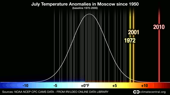
Figure 1 - Probability of July average temperature anomalies in Moscow, Russia since 1950. This image shows that the average temperature in Moscow for July 2010 was significantly hotter than in any year since 1950. Credit: Claudia Tebaldi and Remik Ziemlinski. From ClimateCentral.org
Earlier statistical work on record-breaking events has shown that for any time series that is stationary (i.e. no trend), the probability of record-breaking falls with each subsequent observation. This is known as the 1/n rule, where n equals the previous number of data in the series. For example, the first observation has a 1-in-1 chance of being the record extreme (100%), the second has a 1-in-2 chance (50%), the third a 1-in-3 chance, and so on.
For climate heat records, the stationarity rule is not apparent, as one might expect in a warming world. Previous work in this area has shown that the slowly warming mean (average) temperature is responsible for this nonstationarity.
Following on from this earlier work, Rahmstorf and Coumou (2011) sought to disentagle the two effects of the mean change in temperature (climate warming), from the random fluctuations of weather, so as to find out the contribution of each to record-breaking. To do this, the study authors turned to Monte Carlo simulations. These are computer-generated calculations which use random numbers to obtain robust statistics. A useful analogy here is rolling a dice. Rolling once tells us nothing about the probability of a six turning up, but roll the dice 100,000 (as in this experiment) and you can calculate the odds of rolling a six.
From the simulations the authors obtain 100 values which represent a 100 year period. Figure 2(A) - 2(C) are the "synthetic" time series, and 2(D), 2(E) are respectively, the 'synthetic' global mean and Moscow July temperature. In all panels the data have been put into a common reference frame (nomalized) for comparison. (See figure 1 for an example of a Gaussian or normal distribution. Noise represents the year-to-year variability).
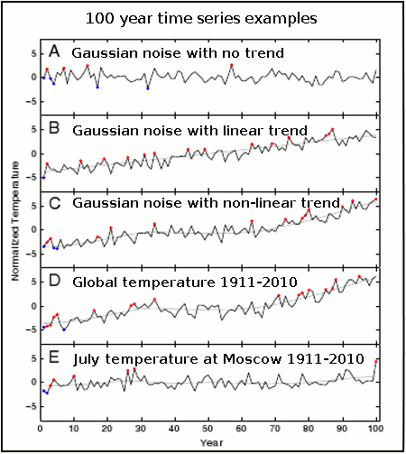
Figure 2 - examples of 100 year time series of temperature, with unprecedented hot and cold extremes marked in red and blue. A) uncorrelated Gaussian noise of unit standard deviation. B) Gaussian noise with added linear trend of 0.078 per year. C) Gaussian noise with non-linear trend added (smooth of GISS global temp data) D) GISS annual global temp for 1911-2010 with its non-linear trend E) July temp at Moscow for 1911-2010 with non-lnear trend. Temperatures are normailzed with the standard deviation of their short-term variability (i.e. put into a common frame of reference). Note: For the Moscow July temperature (2E) the long-term warming appears to be small, but this is only because the series has been normalized with the standard deviation of that records short-term variability. In other words it simply appears that way because of the statistical scaling approach - the large year-to-year variability in Moscow July temperatures makes the large long-term increase (1.8°C) look small when both are scaled. Adapted from Rahmstorf & Coumou (2011)
Initially, the authors ran the Monte Carlo simulations under 3 different scenarios, the first is for no trend (2[A]), with a linear trend (2[B]) and a nonlinear trend (2[C]). The record-breaking trends agree with previous statistical studies of record-breaking namely that: with no trend the probability of record-breaking falls with each observation (the 1/n rule), and with a linear trend the probability of record-breaking gradually reduces until it too exhibits a linear trend. With a non-linear trend (2[C]), the simulations show behaviour characteristic of the no-trend and linear trend distibutions. Figures 2(D) and 2(E) are the actual GISS global and Moscow July temperatures respectively.
Next, the authors then looked at both the GISS global and Moscow July temperature series to see whether they exhibited a gaussian-like distribution (as in the 'lump' in figure 1). They did, so this supports earlier studies indicating that temperature deviations are fluctuating about, and shifting with a slowly moving mean (as in the warming climate). See figure 3 below.

Figure 3 -Histogram of the deviations of temperatures of the past 100 years from the nonlinear climate trend lines shown in Fig. 2(D) and (E) together with the Gaussian distributions with the same variance and integral. a) Global annual mean temperatures from NASA GISS, with a standard deviation of 0.088 ºC. (b) July mean temperature at Moscow station, with a standard deviation of 1.71 ºC. From Rahmstorf & Coumou (2011)
Although the authors calculate probabilities for a linear trend, the actual trend for both the global, and Moscow July temperature series is nonlinear. Therefore they separated out the long-term climate signal, and the weather-related annual temperature fluctuation, which gave them a climate 'template' on which to run Monte Carlo simulations with 'noise' of the same standard deviation (spread of annual variability from the average, or mean). This is a bit like giving the Earth the chance to roll the 'weather dice' over and over again.
From the simulations with, and without the long-term trend, the authors could then observe how many times a record-breaking extreme occurred.
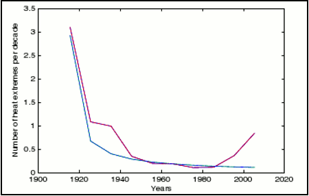
Figure 4 -Expected number of unprecedented july heat extremes in Moscow for the past 10 decades. Red is the expectation based on Monte Carlo simulations using the observed climate trend shown in Figure 2(E). Blue is the number expected in a stationary climate (1/n law). Warming in the 1920's and 1930's and again in the last two decades increases the expectation of extremes during those decades. From Rahmstorf and Coumou (2011)
A key finding of the paper was that if there are large year-to-year non-uniform fluctuations in a set of observations with a long-term trend, rather than increasing the odds of a record-breaking event, they act to reduce it because the new record is calculated by dividing the trend by the standard deviation The larger the standard deviation the smaller the probability of a new extreme record.
This can be seen by comparing the standard deviation of the NASA GISS, and Moscow July temperature records (figure 3), plus figure 2(D) and [E]). As the GISS global temperature record has a smaller standard deviation (0.088°C) due to the smaller year-to-year fluctuations in temperature, you will note in figure 2(D) that it has a greater number of record-breaking extremes than the Moscow July temperature record over the same period (2[E]). So, although the long-term temperature trend for Moscow in July is larger (100 year trend=1.8°C), so too is the annual fluctuation in temperature (standard deviation=1.7°C), which results in lower probability of record-breaking warm events.
Interestingly it's now plain to see why the MSU satellite temperature record, which has a large annual variability (large standard deviation, possibly from being overly sensitive to La Niña & El Niño atmospheric water vapor fluctuations) still has 1998 as it warmest year, whereas GISS has 2005 as it's warmest year (2010 was tied with 2005, so is not a new record). Even though the trends are similar in both records, the standard deviation is larger in the satellite data and therefore the probability of record-breaking is smaller.
The results of this paper directly contradict the findings of Dole (2011) who discounted a global warming connection with the 2010 Russian heatwave. Rahmstorf & Coumou (2011) demonstrate that the warming trend from 1980 onwards (figure 4) greatly increased the odds of a new record-breaking warm extreme, and in fact should have been anticipated.
It turns out that Dole (2011) failed to account for a quirk in the GISS Moscow station data which had wrongly applied the annual urban heat island (UHI) adjustment for the monthly July temperatures, when UHI is a winter phenomenon in Moscow. This meant that the large warming trend evident there in July had been erroneously removed. This was confirmed by looking at Remote Sensing Systems (RSS) satellite data over the last 30 years, which shows a strong warming trend in Moscow July temperatures. See Real Climate post "The Moscow Warming Hole" for detail, and note Figure 5 below.
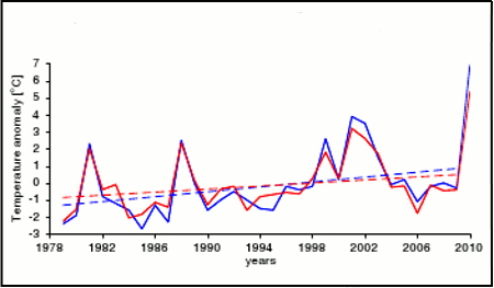
Figure 5 - Comparison of temperatues anomalies from RSS satellite data (in red) over the Moscow region versus Moscow station data (in blue). Solid lines shows the average July value for year, whereas the dashed lines show the linear trend for 1979-2009. Satellite data have a trend of 0.45°C per decade, as compared to 0.72°C per decade for the Moscow station data.
Using the GISS data from 1911-2010 (a nonlinear trend), the authors calculate a 88% probability the extreme Russian heatwave (a record in the last decade of the series) was due to the warming trend. Clearly the summer temperatures for July 2010 in Moscow were a massive departure from normal, and including them would create bias, so the study authors exclude 2010 from their analysis, and re-calculate for 1910-2009. They found a 78% probability the freak heatwave was due to warming, and extending their analysis back to include the entire GISS temperature observations (1880 -2009), they found an 80% probability.
So to sum up:
Posted by Rob Painting on Friday, 11 November, 2011
 |
The Skeptical Science website by Skeptical Science is licensed under a Creative Commons Attribution 3.0 Unported License. |