James Hansen, M. Sato and R. Ruedy have posted a new paper to their website. It has not been peer reviewed yet, but will eventually be published with some changes. Hansen et al. (2011) analyzes surface temperature data and quantify the number of very hot and very cold summers and winters.
Hansen et al. use the period 1951-1980 to calculate an average temperature for each location. Then the difference between a measured temperature and the average is calculated and called the anomaly. For example, if the average temperature in a place is 10°C, and one day records 15°C, then the anomaly is +5°C. The anomaly makes it easier to compare temperature records in different locations.
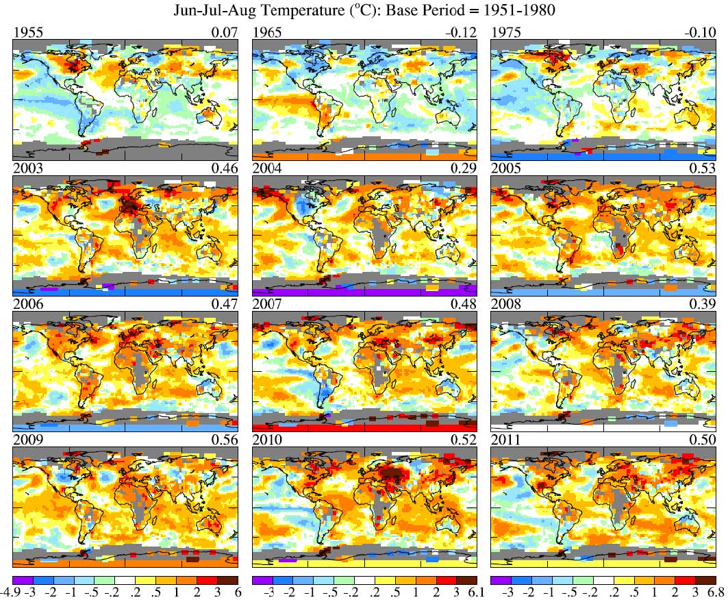
Where there are data, this allows maps of hotter-than-normal and colder-than-normal temperatures to be created, as in Figure 1.

Figure 1. Jun-Jul-Aug surface temperature anomalies in 1955, 1965, 1975 and the past nine years relative to 1951-1980 mean. Number on upper right is the global (area with data) mean.
Hansen et al. calculate the standard deviation of the temperature at each location. The standard deviation of the data measures how much the temperature normally varies about the average at that location. They take the temperature anomaly at each location and divide it by the standard deviation for that location to determine how many standard deviations away from normal the temperatures at that location were. This allows Hansen to compare how much the temperature has changed due to Global Warming (the anomaly) to how much the temperature normally varies at each location.
If the temperature anomaly follows a normal Gaussian curve, the number of data points that are more than one standard deviation (abbreviated as σ) from the average can be calculated. In a normal distribution of the data, 68% of the data points fall within 1σ of the average value: 34% higher than average, 34% lower than average. Only 2.3% of data points are expected to be over +2σ and only 0.13% over +3σ from the average (the same number would be -2σ and -3σ). When Hansen looked at the data from 1951 to 1980, the distribution of data was very similar to a normal distribution. The data from 2003-2011 tell a different story. Here is the data for June-July-August showing 1955, 1965, 1975 and 2003-2011.

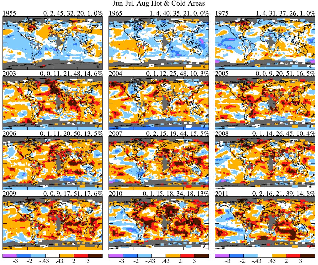
Figure 3. Jun-Jul-Aug surface temperature anomalies in 1955, 1965, 1975 and 2003-2011 relative to 1951-1980 mean temperature in units of the local standard deviation of temperature.
In this graph the gray areas have no data. The dark red areas are +2σ hotter than normal and the black areas are +3σ hotter than normal. Blue and purple areas are cooler than normal. From 1955-1975 there are similar amounts of blue and orange, with little red and no black. From 2003-2011 there is not much blue. Orange, red and black predominate. Can we quantify the amount of difference? Hansen has tallied the areas of each σ in the upper corner of each section of the figure, but I find the graph below easier to read.
Figure 5. Area of the world covered by temperature anomalies in the categories defined as hot (σ > 0.43), very hot (σ > 2), and extremely hot (σ > 3), with analogous divisions for cold anomalies. These anomalies are relative to 1951-1980 climatology with σ from the detrended 1981-2010 data, but results are similar for the alternative choices for standard deviation.
In Figure 5, the center graph is “normal” temperatures, within 0.43σ of the average temperature. We expect 33% of the measurements to fall in this range. Hot (Cold) is defined as temperatures greater (less) than 0.43σ. We expect each of these 33% of the time. Very Hot (Very Cold) is greater (less) than 2σ, expected 2.3% of the time and Extremely Hot is greater than 3σ, expected only 0.13%. The Hot data include the Very Hot points and the Very Hot data include the Extremely Hot points so the lines do not add up to 100% (Hot + Normal + Cold = 100%). We will look at the June-July-August temperatures (December, January and February are slightly different, the reason is discussed in the paper).
From 1950 to 1980 normal temperatures, cold and hot are all present about 33% of the time as expected. There is little Very Hot or Very Cold. The Nauties are completely different. Normal and Cold have dropped to 20 and 15% respectively and Hot has risen to about 66%. In 2010, Very Hot (+2σ) occurred over 31% of the Earths surface and Extremely Hot (+3σ) occurred over 13% of the Earth’s surface, while the corresponding Very Cold and Extremely Cold were 1% and 0%.
Hansen says:
“The most dramatic and important change of the climate dice is the appearance of a new category of extreme climate outliers. These extremes were practically absent in the period of climatology, covering much less than 1% of Earth's surface. Now summertime extremely hot outliers, more than three standard deviations (σ) warmer than climatology, typically cover about 10% of the land area. Thus there is no need to equivocate about the summer heat waves in Texas in 2011 and Moscow in 2010, which exceeded 3σ – it is nearly certain that they would not have occurred in the absence of global warming. If global warming is not slowed from its current pace, by mid-century 3σ events will be the new norm and 5σ events will be common.”
Looking at Figure 3, we see in 2010 that Moscow was in the middle of a large black spot of +3σ, while in 2011 Texas was in the middle of a similar spot. Europe had its time in the heat in 2003. All these outliers were absent from 1950-1980. People who continue to deny that extreme heat is caused by AGW need to look carefully at these graphs. These extreme weather events were not normal; they are directly caused by AGW. They are becoming normal now. In 2010, 17% of the world’s land area was Extremely Hot (data not shown). In the 1960s there were virtually zero Extremely Hot areas.
By doing an analysis of the entire globe at once, Hansen has gotten around the problem of attribution of a single event. Global data, averaged over several months, allows Hansen to conclude that most of these events would not have happened without AGW. Extremely Hot events, even for a single summer, kill established trees, permanently damage ecosystems and cause severe economic distress. Praying for rain (as recommended by the Governor of Texas) is unlikely to correct the problem as long as we continue to emit large amounts of climate changing gasses.
Posted by michael sweet on Tuesday, 3 January, 2012
 |
The Skeptical Science website by Skeptical Science is licensed under a Creative Commons Attribution 3.0 Unported License. |