"An area and distance weighted analysis of the impacts of station exposure on the U.S. Historical Climatology Network temperatures and temperature trends"
Paper authors: A. Watts, E. Jones, S. McIntyre and E. R. Christy
In an unpublished paper, Watts et al. raise new questions about the adjustments applied to the U.S. Historical Climatology Network (USHCN) station data (which also form part of the GHCN global dataset). Ultimately the paper concludes "that reported 1979-2008 U.S. temperature trends are spuriously doubled." However, this conclusion is not supported by the analysis in the paper itself. Here we offer preliminary constructive criticism, noting some issues we have identified with the paper in its current form, which we suggest the authors address prior to submittal to a journal. As it currently stands, the issues we discuss below appear to entirely compromise the conclusions of the paper.
In reaching the conclusion that the adjustments applied to the USHCN data spuriously double the actual trend, the authors rely on the difference between the NCDC homogenised data (adjusted to remove non-climate influences, discussed in detail below) and the raw data as calculated by Watts et al. The conclusion therefore relies on an assumption that the NCDC adjustments are not physically warranted. They do not demonstrate this in the paper. They also do not demonstrate that their own ‘raw’ trends are homogeneous.
Ultimately Watts et al. fail to account for changing time of observations, that instruments change, or that weather stations are sometimes relocated, causing them to wrongly conclude that uncorrected data are much better than data that takes all this into account.
The purpose of the paper is to determine whether artificial heat sources have biased the USHCN data. However, accounting for urban heat sources is not the only adjustment which must be made to the raw temperature data. Accounting for the time of observations (TOB), for example, is a major adjustment which must be made to the raw data (i.e. see Schaal et al. 1977 and Karl et al. 1986).
For example, if observations are taken and maximum-minimum thermometers reset in the early morning, near the time of minimum temperature, a particularly cold night may be double-counted, once for the preceding day and once for the current day. Conversely, with afternoon observations, particularly hot days will be counted twice for the same reason. Hence, maximum and minimum temperatures measured for a day ending in the afternoon tend to be warmer on average than those measured for a day ending in the early morning, with the size of the difference varying from place to place.
Unlike most countries, the United States does not have a standard observation time for most of its observing network. There has been a systematic tendency over time for American stations to shift from evening to morning observations, resulting in an artificial cooling of temperature data at the stations affected, as noted by Karl et al. 1986. In a lecture, Karl noted:
"There is practically no time of observation bias in urban-based stations which have taken their measurements punctually always at the same time, while in the rural stations the times of observation have changed. The change has usually happened from the afternoon to the morning. This causes a cooling bias in the data of the rural stations. Therefore one must correct for the time of observation bias before one tries to determine the effect of the urban heat island"
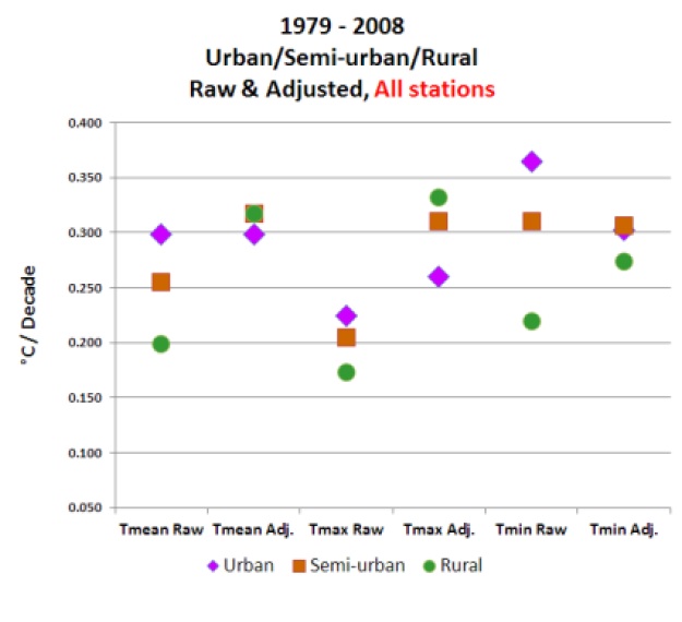
Note in Watts Figure 16, by far the largest adjustments (in the warming direction) are for rural stations, which is to be expected if TOB is introducing a cool bias at those stations, as Karl discusses.
As Zeke Hausfather has also discussed, the biggest network-wide inhomogeneity in the US record is due to the systematic shift from manually-read liquid-in-glass thermometers placed in a louvred screen (referred to in the U.S. as a Cotton Region Shelter and elsewhere as a Stevenson screen) to automated probes (MMTS) in cylindrical plastic shelters across large parts of the network in the mid- to late-1980s. This widespread equipment change caused an artificial cooling in the record due to differences in the behaviour of the sensors and the sheltering of the instruments. This is discussed in a number of papers, for example Menne et al. 2009 and 2010, and like TOB does not appear to be accounted for by Watts et al.
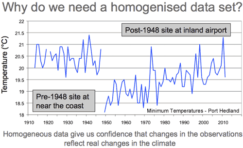
Additionally, the Watts paper does not show how or whether the raw data were adjusted to account for issues such as sites closing or moving from one location to another. The movement of a site to a location with a slightly different mean climatology will also result in spurious changes to the data. The Watts paper provides no details as to how or whether this was accounted for, or how the raw data were anomalised.

Quite simply, the data are homogenised for a reason. Watts et al. are making the case that the raw data are a ‘ground truth’ against which the homogenisations should be judged. Not only is this unsupported in the literature, the results in this paper do nothing to demonstrate that. It is simply wrong to assume that all the trends in raw data are correct, or that differences between raw and adjusted data are solely due to urban heat influences. However, these wrong assumptions are the basis of the Watts conclusion regarding the 'spurious doubling' of the warming trend.
The conclusion regarding the lower surface temperature warming trend is also at odds with the satellite temperature data. Over the continental USA (CONUS), satellites show a 0.24°C per decade warming trend over the timeframe in question. According to Klotzbach et al. (2010), which the Watts paper references, there should be an amplification factor of ~1.1 between surface and lower troposphere temperatures over land (greater atmospheric warming having to do with water vapor amplification). Thus if the satellite measurements were correct, we would expect to see a surface temperature trend of close to 0.22°C per decade for the CONUS; instead, the Watts paper claims the trend is much lower at 0.155°C per decade.
This suggests that either the satellites are biased high, which is rather implausible (i.e. see Mears et al. 2011 which suggests they are biased low), or the Watts results are biased low. The Watts paper tries to explain the discrepancy by claiming that the amplification factor over land ranges from 1.1 to 1.4 in various climate models, but does not provide a source to support this claim, which does not appear to be correct (this may be a reasonable range for global amplification factors, but not for land-only).
A discussion between Gavin Schmidt and Steve McIntyre on this subject led to the conclusion that the land-only amplification factor falls in the range of 0.78 to 1.23 (average over all global land areas), with a model mean close to 1 (using a script developed by McIntyre on 24 different models). Note that McIntyre is a co-author of Watts et al., but has only helped with the statistical analysis and did not comment on the whole paper before Watts made it public. We suggest that he share his land-only amplification factor discussion with his co-authors.
Another important consideration is that the amplification factor also varies by latitude. For example Vinnikov et al. (2005) found that at the CONUS latitude (approximately 40°, on average), models predict an amplification factor of approximately 1 (see their Figure 9). Note that this is the amplification factor over both land and ocean at this latitude. Since the amplification factor over land is less than that over the oceans, this suggests that the amplification factor over the CONUS land may even be less than 1.
Combining the latitude and land-only status of the CONUS, the amplification factor may very well be less than 1, but a range of values significantly lower than the 1.1 to 1.4 range used in the Watts paper would be reasonable.
Note also that as discussed above, the satellite data (like all data) are imperfect and are not a 'gold standard'. They are a useful tool for comparison in this study, but the satellite trends should not be assumed to be perfect measurements.
Watts et al. compare the best sited Class 1 and 2 stations (using their categorisation) to the total homogenised network. Strictly speaking, this is comparing apples and oranges; Watts' data are an inhomogeneous sub-sample of the network compared to a homogeneous total network. In practice, this methodological error doesn’t make much difference, since the homogenisation applied by NCDC produces uniform trends in all of the various classes.
However the use of a smaller network has disadvantages. When taking a gridded average of a sparse network, the impact of inhomogeneities is likely amplified and the overall uncertainty of variability and change in the timeseries increases.
The Class 1 & 2 sites used by Watts in this context represent just 20% of all the total CONUS network. The comparison of the raw Class 1 & 2 sites with the same network of homogenised data in Watts' own Figure 18 indicates likely inhomogeneities in that raw data. Watts et al. argue that the raw and adjusted Class 1 & 2 trends in Figures 18a and 18b are so different because "well sited stations are adjusted upward to match the already-adjusted poor stations," but this is simply not how the homogenization process is done. In reality the difference is likely due to the biases we have discussed above, indicating that the Watts raw data is inhomogeneous and influenced by these non-climate effects.
Determining whether or not the Class 1 & 2 raw data is homogeneous is therefore a key requirement of a revised manuscript. And since the Class 1 & 2 sites have been selected for good exposure, Watts et al. would need to show the cause of any statistical discontinuities that they find. This work has already been done by NCDC in the Menne at al. papers, which show influences from the range of factors discussed above, and not just urban influence.
The Watts final conclusion that adjusted temperature trends are 'spuriously doubled' (0.155°C vs. 0.309°C per decade raw vs. adjusted data) relies on a simple assumption — that the raw data must be correct and the homogenised data incorrect. There is no a priori basis for this assumption and it is unsupported by the literature.
While Watts et al. identify possible issues concerning the adjustments applied to station temperature records, it wisely makes no attempt to assess the global impact of the adjustments, which are beyond the scope of the work. Nonetheless, this is a significant question from a public interest perspective.
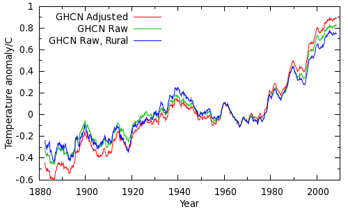
In order to answer this question, we willl try and estimate the maximum possible impact of station adjustments on the instrumental temperature record. To minimise the warming signal, we will use the simplest method for calculating a global temperature average - the CRU method, which is known to yield poor coverage at high latitudes and hence underestimate recent warming. Further, we'll assume that entirety of the data adjustments are wrong (ignoring proven bias corrections such as TOB). If we calculate land temperature averages from both the raw and adjusted data, we can see how much difference the adjustments make. The result is shown in the figure below (red and green lines).

Just to be absolutely sure, we can do a further calculation using just rural unadjusted data (using the GHCN station classifications) - the blue line.
While the adjustments do make a difference, the difference is small compared to the overall warming signal since 1979. Using a more sophisticated temperature calculation reduces this difference. Furthermore, we are only looking at land temperatures - 30% of the planet. Including the remaining 70% of the planet (the oceans which, if not precisely rural, are certainly not urban!) dramatically reduces the remaining impact of the GHCN adjustments. Indeed, comparison of warming trends over the oceans and over large inland lakes (including the North American Great Lakes) shows a high degree of consistency with terrestrial trends. Warming over the oceans and lakes is presumably not due to urbanisation.
The entire CRU-type calculation requires 65 lines of python code (by comparison, a modern airliner requires upwards of a million lines of code to fly). The code is available below.
Show code
Many others have done this comparison, including Caerbannog and Zeke Hausfather. Fawcett et al (2012) provide a comprehensive assessment of the sensitivity of Australian temperature trends to network and homogenisation choices, including comparison with an unhomogenised gridded analysis of Australian temperatures. Furthermore, the BEST project has obtained a similar result with a different, independent implementation of the station homogenization algorithm. It would be surprising if an independent approach were to yield a similar but incorrect result by chance.
Do the overall adjustments make a difference? Yes. Are they justified? Yes, according to the body of scientific literature. Watts raises a scientific issue, but one which only affects part of the adjustment. Does it matter? Not very much. Even if the entirety of the adjustments were wrong, we still see unprecedented warming over the past 40 years. And there is certainly not a factor of two difference between global warming trends in the raw and adjusted data.
It's worth noting that Peter Thorne of NCDC was interviewed by Andrew Revkin, and discussed three papers which NCDC has recently published (see here, here, here). In the first of those linked papers, they actually concluded that there likely remains a residual cool bias in the adjusted data, and that the adjusted data are consistent with reanalysis data (detailed in the third linked paper). Watts et al. do not address these papers. Ironically Watts responded to that interview by saying that Thorne needs to get out into the real world, but it is Watts et al. who have not accounted for real world effects like TOB, station movement, instrument changes, etc.
In its current form, the Watts paper contains little in the way of useful analysis. There are too many potential sources of bias which are not accounted for, too many apples-to-oranges comparisons, and they cannot draw any conclusions about urban heat influences until their data are homogenized and other non-climate influences are removed.
The primary conclusion of the paper, aside from not being supported by the analysis, is simply implausible. The CONUS surface warming trend proposed by the Watts paper appears to be inconsistent with the satellite observations, and overall global trends in raw data do not differ dramatically from those in the adjusted data. Comparing raw to adjusted data globally shows a rather small difference in long-term trends; far smaller than a factor of two.
The flaws we have identified entirely compromise the conclusions of the paper. Ultimately Watts et al. assume that all adjustments are 'spurious' unless due to urban heat influences, when in fact most of their identified discrepancy likely boils down to important adjustments for instrumental changes, TOB, and other influences they have not accounted for in their analysis. Watts et al. attempt to justify their assumption by asserting "well sited stations are adjusted upward to match the already-adjusted poor stations," but this is simply not how the homogenization process is done.
Fortunately McIntyre has acknowledged that TOB must be considered in their analysis, as has Watts, which is a good start, but they must also account for the other biases noted above in order to draw any valid conclusions about urban heat influences.
In conclusion, Watts et al. of course deserve the right to try to make their case in the peer-reviewed literature, however implausible that case appears to be. Therefore, we hope they will consider addressing the important concerns detailed above before they submit the paper to a journal. Otherwise we suspect the paper will not fare well in the peer review process. With said caveats carefully addressed and the conclusions amended if and where necessary, the paper has the potential to be a useful contribution to the climate science literature.
Posted by dana1981 on Thursday, 2 August, 2012
 |
The Skeptical Science website by Skeptical Science is licensed under a Creative Commons Attribution 3.0 Unported License. |