This is a guest post by KK Tung, who requested the opportunity to respond to the SkS post Tung and Zhou circularly blame ~40% of global warming on regional warming by Dumb Scientist.
The observed global-mean temperature has gone through a number of ups and downs since 1850, which is the beginning of the available global temperature record. Our recent paper of Tung and Zhou [2013] in Proceedings of National Academy of Science (PNAS) was the latest among a large body of published literature on the evidence of a multidecadal oscillation that can be seen in the global-mean surface temperature record. We further reported a quantitative analysis (multiple linear regression (MLR)) using the global (not regional) temperature data (HadCRUT4) that attributed a warming rate of 0.07-0.08 °C/decade to net anthropogenic forcing. That warming rate has been steady for the past 100 years, through the ups and downs of about 30-year duration, which we attributed to the Atlantic Multi-decadal Oscillation (AMO). In this view, the anthropogenic warming has not stalled in the past decade and half, nor has it accelerated in the previous three decades. I thank Skeptical Science for giving me this opportunity to explain in a more understandable way some underlying issues that have caused confusion to nonspecialists.
How can the anthropogenic warming be approximately linear in time when we know that atmospheric CO2 has been measured to increase almost exponentially? Implicit in that statement is the expectation that the warming (i.e. the rate of surface temperature increase) should follow the rate of increase of greenhouse gas concentration in the atmosphere. This rather common expectation is incorrect. An accessible reference is that from Britannica.com: “Radiative forcing caused by carbon dioxide varies in an approximately logarithmic fashion with the concentration of that gas in the atmosphere. The logarithmic relationship occurs as the result of a saturation effect wherein it becomes increasingly difficult, as CO2 concentrations increase, for additional CO2 molecules to further influence the ‘infrared window’ (a certain narrow band of wavelengths in the infrared region that is not absorbed by atmospheric gases)”.

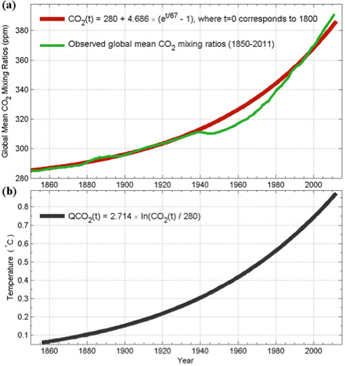
Figure 1. (a) the measured atmospheric concentration of carbon dioxide in green and the fitted smooth function in red. (b) the logarithm of the red curve in (a). The constant multiplier in front converts it to the global mean temperature; details of that MLR analysis are not discussed here to avoid confusion.
Figure 1a shows that the well measured CO2 concentration (in green) can be fitted to an exponential function plus a constant preindustrial value (in red). So it is true that one can claim that the carbon dioxide concentration in the atmosphere has increased at an exponential rate. Normally the logarithm of an exponential function in time is linear in time. However the fit of CO2 has a constant in additional to the exponential, and so its logarithm is slightly more curvy than linear. Nevertheless it can still be regarded as almost linear over multidecadal intervals to within 0.1 °C. Logarithm of that function is shown in Figure 1b as QCO2, which represents the radiative heating from CO2. The exponential growth of the CO2 after 1950 is much muted in the logarithm (taking into account the fact that the vertical scale is in small 0.1°C increments.
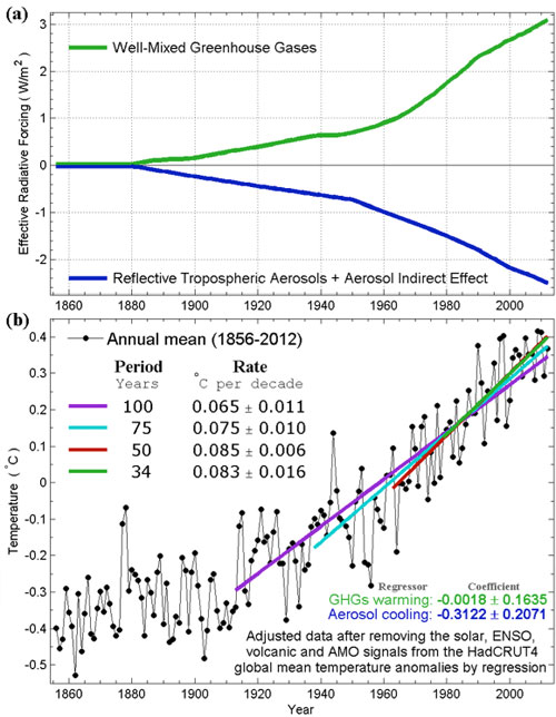
The real situation is more complicated than indicated by these simple functions, because the net anthropogenic forcing is the sum of radiative heatings from individual greenhouse gas concentrations and tropospheric sulfate aerosol cooling (man-made pollution). We show in Figure 2a the sum of radiative heating from all well-mixed greenhouse gases in green and the sum of radiative cooling from tropospheric aerosol effects in blue. Because some of the greenhouse gases such as methane are more powerful radiatively than carbon dioxide, one cannot simply take the logarithm of the sum of the greenhouse gas concentrations to arrive at the total heating rate from them. They need to be calculated individually. These calculated radiative heating rates are available from NASA's Goddard Institute for Space Studies (GISS) at http://data.giss.nasa.gov/modelforce/, and have been used in the GISS model, one of the models participating in IPCC studies. As shown in Figure 2a, the green line is quite nonlinear and shows the acceleration of greenhouse gas forcing after 1950 referred to by DS, but the aerosol cooling also increased after 1950. The net anthropogenic forcing is the small difference of the two large terms. The near cancellation by the two anthropogenic components may be one of the explanations of why the warming deduced by Tung and Zhou is smaller than the response expected from greenhouse gas warming alone. Because the aerosol cooling part is uncertain, we actually do not know what the net anthropogenic forcing looks like. There is no obvious argument that one can appeal to on what the expected warming should be. There is nothing obviously wrong if the anthropogenic warming is found to be almost linear in time. This is the first point I would like to make.
(A side comment: Depending on the exact form of the aerosol cooling adopted, the net anthropogenic forcing is different from model to model. Although you probably cannot see it just by eye-balling the two curves in Figure 2a, their difference actually is nonlinear, with accelerating heating after 1978, allowing the GISS model to produce the accelerated warming after 1978 from anthropogenic forcing alone. Other groups adopt somewhat different time dependent shape of net anthropogenic forcing. See here and here.
Analysis of models by several authors showed that there was a large range of net anthropogenic forcing adopted by models participating in IPCC assessment reports, with a tendency for the models with higher climate sensitivity to adopt a lower net forcing and less sensitive models to adopt a higher net forcing.)

Figure 2. (a) Radiative forcing of various anthropogenic components. (b) Results of Multiple Linear Regression using natural and anthropogenic regressors. Adjusted temperature, which is the same as the combined response to the anthropogenic forcing plus the Residual is shown. This multiple linear regression using two highly collinear regressors is not recommended, but nevertheless yields approximately the same result for the adjusted temperature trend.
One common way to deduce the anthropogenic warming signal from observed data is to remove all other known natural influences, such as El Nino, volcanic aerosols, solar forcing (cyclic and secular) and the AMO. These are called the predictors or regressors. What remains are random climate noise, and the net anthropogenic warming rate. We call the sum of the two the “adjusted data”, following Foster and Rahmstorf [2011] . The MLR model for the observed temperature T(t) is:

The MLR procedure assumes the form for the predictors and tries to fit the observed temperature with them using the least-squares best fit. The model is successful if the procedure yields a Residual(t) that contains only climate noise, but often it also contains some trend. When that happens it is telling us that the assumed trend in the anthropogenic component (e*Anthro(t)) is probably not correctly giving the anthropogenic trend consistent with the observed temperature.
The adjusted data can be viewed as the temperature with natural variations removed. Because the adjusted temperature can also be expressed as
![]()
the deduced anthropogenic trend can be corrected by adding the trend in the Residual to e*Anthro(t). It turns out that this trend deduced from the Adjusted temperature is not always the same that in e*Anthro(t). This procedure of deducing the trend from Adjusted temperature is actually not sensitive to the assumed form of Anthro(t), as long as it has a long-term trend: When the assumed Anthro(t) has a too large a trend after 1978 compared to before 1978, for example, the Residual (t) will show a negative trend after 1978 and a positive trend before that time. See the example discussed in Zhou and Tung [2013] . Since we do not know a priori what the form of net anthropogenic forcing is because of its large uncertain tropospheric sulfate aerosol component, to be agnostic we used a linear function for Anthro(t) in the intermediate step as a “placeholder”. That was probably the source of the circular argument criticism from DS: “Tung and Zhou implicitly assumed that the anthropogenic warming rate is constant before and after 1950, and (surprise!) that's what they found. This led them to circularly blame about half of global warming on regional warming.” It is important to note that the trend we were talking about is the trend of the Adjusted data, and not the presumed anthropogenic predictor.
We will next show that we get approximately the same result using more nonlinear placeholders for the anthropogenic predictor. In the first example, we proceed to do a MLR analysis using the two anthropogenic predictors: one the nonlinear green line and the other the blue line in Figure 2a, and let the MLR procedure adjust the proportions of the two to get a best fit. This is probably what nonspecialists would find most natural and expect us to do (but specialists know not to do). After the multiple regression analysis is done, the adjusted data is reconstructed by adding the residual to the sum of the two regressed anthropogenic responses. This is shown in Figure 2b. The regression coefficient of greenhouse gas warming is shown as “warming” and the aerosol cooling is shown as “cooling”. The multiple regression analysis is confused by the two highly correlated anthropogenic regressors (this is the well-known problem of collinearity), producing a “warming” that is negative and a “cooling” that is positive. This is not surprising given how close the two curves look in Figure 2a. Nevertheless, the combination of the two responses is robust. When combined to yield the adjusted data, the 100-year, 50-year and 34-year linear trends are still rather steady at ~0.07-0.08°C/decade as shown by the dots in Figure 2b and the trends fitted through them. The result is very close to that found in Tung and Zhou [2013] using a linear predictor as a placeholder. We have tried many other predictors with similar results. Using a nonlinear anthropogenic regressor would still yield an almost linear trend for the past 100 years, if the Residual is added back. And so this procedure is not circular. This is the second point I am trying to make.
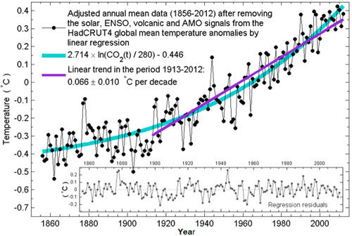
Of the different regressors we tried the single anthropogenic regressor that is closest to the final adjusted data turns out to the QCO2(t) function given in Figure 1b. This is shown in Figure 3. The difference between the adjusted data and the QCO2 regressor is the Residual, which is shown in the inset. Except for s a minor negative trend in the last decade in the Residual, it is almost just noise. So the MLR with QCO2 as the anthropogenic regressor is successful. That small negative trend in the Residual, when added back to QCO2, yields a more linear trend in the adjusted data, similar to what we found in Tung and Zhou and in Figure 2b here. (The physical interpretation of why the net anthropogenic warming appears to follow the radiative heating by CO2 alone and with so little lag between forcing and response is rather tricky and will not be discussed here.)

Figure 3. Adjusted data shown in dots, obtained by a MLR using QCO2 as the anthropogenic predictor. The QCO2 is superimposed. The Residual is shown in the inset
Because of the page limitation of PNAS, a review of the physics of the AMO by other researchers is necessarily brief, with fuller discussions given in the references quoted. Even so, our PNAS paper has the following paragraph on the physical mechanism of the AMO, which Dumb Scientist apparently missed: “The phenomenon likely involves thermohaline circulation variability in the Atlantic Ocean. As described in Dima and Lohmann [2007 ]; Semenov et al. [2010] , the negative feedbacks between the strength of the thermohaline circulation which brings warm sea-surface temperature (SST) to the North Atlantic, and the Arctic ice melt in response to the warm SST, which, because of reduced deep-water formation, then slows the strength of the thermohaline circulation after a delay of 20 years, together create the restoring force responsible for the oscillation. Recently a 55-80-year AMO has been model simulated as arising from the variability of the meridional overturning circulation in the Atlantic Wei and Lohmann [2012] .”
As I have now exceeded the recommended length for the post, I hope in a second post to give a more detailed review of the physical mechanisms of the AMO (noting that the science is not yet settled), its relation to the Atlantic Meridional Overturning Circulation, the choice of the AMO Index (whether the detrending should be point by point or by the global mean), and why the claim that the observed multidecadal variability can be simulated using time-varying aerosols may not be consistent with the observed data.
Dima, M. and G. Lohmann, 2007: A Hemispheric Mechanism for the Atlantic Multidecadal Oscillation. Journal of Climate, 20, 2706-2719.
Foster, G. and S. Rahmstorf, 2011: Global temperature evolution 1979-2010. Environmental Research Letters, 6, 1-8.
Semenov, V. A., M. Latif, D. Dommenget, N. Keenlyside, A. Strehz, T. Martin, and W. Park, 2010: The impact of North Atlantic-Arctic multidecadal variability on Northern Hemisphere surface air temperature. J. Climate, 23, 5668-5677.
Tung, K. K. and J. Zhou, 2013: Using Data to Attribute Episodes of Warming and Cooling in Instrumental Record. Proc. Natl. Acad. Sci., USA, 110.
Wei, W. and Lohmann, 2012: Simulated Atlantic Multidecadal Oscillation during the Holocene. J. Climate, doi:10.1175/JCLI-D-11-00667.1.
Zhou, J. and K. K. Tung, 2013: Deducing the multi-decadal anthropogenic global warming trend using multiple regression analysis. J. Atmos Sci, 70, 3-8.
Posted by KK Tung on Thursday, 11 April, 2013
 |
The Skeptical Science website by Skeptical Science is licensed under a Creative Commons Attribution 3.0 Unported License. |