The worldwide success of books like The Guinness Book of Records is an example of human fascination with record-breaking – the smallest, fastest, farthest, the first etc. The frequency and size of records can tell us something about the underlying process. For example, the world mile record was broken on average once every 3 years between 1913 and 1999, by about 1 second per record. The shift in dominance of middle distance running from the Anglophone countries to Africa has meant the record has only been broken once since 1993.
This post describes a method of recording and graphically presenting successive annual counts of record-breaking months by temperature, e.g. the warmest or the coldest since records were kept, over more than one database. The rate of appearance of record-breaking (warmest or coldest) months intuitively provides a signal of climate change complementary to the usual temperature data. See the “Further Reading” section at the end of the post.
Such data of maximum or minimum records are quite useful as they might, for example, provide evidence of a warming (or cooling) climate, when the temperature data is apparently static over short periods. As we will see, such is what has occurred in the 2000s.
Steps to follow:
(1) Download monthly climate data into a spreadsheet, either the raw data or the temperature anomaly. For easier manipulation, re-arrange the data with successive years in rows underneath each other, and the months in 12 columns, from January to December.
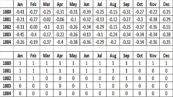
(2) Create a second matrix of rank numbers. In Excel, the RANK function will return the ranking of each monthly temperature datum since the first datum was recorded i.e. the top month in the column. Consult the Excel Help to tell you how to use RANK to find the minimum records, which you can do in a separate worksheet. The IF function can be used to set all ranks, other than the one of interest, to 0. Figure 1 shows the result for the first four years, using GISS data for an example.
(3) In a further column to the right, simply add the number of record months in each year.
(4) If using more than one database, an average is taken. If, for 1960, the GISS database shows 1 new record month, the NOAA database shows 0, and the HADCRUT database shows 1, it is counted as average = 0.66 for 1960, and entered into a score of average yearly record months, which you can keep in another column.
(5) You now have two columns, each of the average maximum and minimum records in each year. You can use two further columns to create running totals of each, and a further column to find the difference between the two running totals.

Figure 1: Conversion of GISS temperature anomaly into a binary indicator of maximum monthly records for first four years.
We intuitively expect that, in a period of warming, there should be more maximum monthly records than minimum, and vice versa in a period of cooling. If we assume that the frequency and duration of warming and cooling periods even out in the long run (natural variation), the running totals of maximum and minimum records should be approximately equal. The differences obtained by subtracting one running total from the other should centre on zero like a sine wave. Figure 2 shows the annual differences in cumulative sums of average new maximum and minimum records in 3 databases (GISS, HADCRUT and NOAA from 1880 to 2010).

Figure 2: Annual differences in cumulative sums of Average Annual Maximum and Minimum Monthly Records. As an example, in 1911 there was an excess of 30 minimum monthly records over maximum, counting since 1880.
Comments:
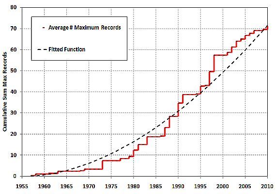
Figure 3 is a chart of the running total of new annual maximum monthly records, starting with the 1955 value set to 0. Note is a non-linear, increasing trend – for each 10 year division, more records are occurring.

Figure 3: Cumulative Change in Annual Average Maximum Monthly Records since 1956. The 1955 value is set = 0.
Comments:
This basic, and even crude, analysis confirms the model of temperature rise given by mainstream climate science. That is no surprise. However, it can be expanded to incorporate natural variation (factors like ENSO and volcanic eruptions) using methods like logistic regression, which is more robust than ordinary least squares. The advantage of this method is that the mathematics of a noisy temperature process has been replaced by the mathematics of a simple stochastic process. Stochastic processes are well understood and used in many situations like monitoring time between crashes of a computer system (in software reliability engineering) or time between events (in health survival analysis).
This analysis undermines, yet again, many of the simplistic contrarian models e.g. that natural variability is driving warming, or that the earth has been cooling in the period 1998-2002. As Professor Richard Lindzen said: “Temperature is always rising and falling”. However, that implies an equalization of maximum and minimum monthly records over a long period. The numbers of minimum monthly records in these global temperature databases has not even been close to numbers of monthly maxima for some time. The last such sequence in these databases ended in 1917, almost one-hundred years ago. The current rate of occurrence of minimum records is 0 per year, and the rate for maximum records is consistently outstripping that of minima by almost 2 per year, and rising.
Further Reading:
How often can we expect a record event? Benestad(2003)
Record-breaking temperatures reveal a warming climate. Wergen(2010)
Detection Probability of Trends in Rare Events: Theory and Application to Heavy Precipitation in the Alpine Region. Frei(2001)
Posted by shoyemore on Tuesday, 15 March, 2011
 |
The Skeptical Science website by Skeptical Science is licensed under a Creative Commons Attribution 3.0 Unported License. |