Climate Science Glossary

Term Lookup

Enter a term in the search box to find its definition.

Settings

Use the controls in the far right panel to increase or decrease the number of terms automatically displayed (or to completely turn that feature off).

Term Lookup

Settings


All IPCC definitions taken from Climate Change 2007: The Physical Science Basis. Working Group I Contribution to the Fourth Assessment Report of the Intergovernmental Panel on Climate Change, Annex I, Glossary, pp. 941-954. Cambridge University Press.

Home Arguments Software Resources Comments The Consensus Project Translations About Support

Bluesky Facebook LinkedIn Mastodon MeWe

Twitter YouTube RSS Posts RSS Comments Email Subscribe


Climate's changed before
It's the sun
It's not bad
There is no consensus
It's cooling
Models are unreliable
Temp record is unreliable
Animals and plants can adapt
It hasn't warmed since 1998
Antarctica is gaining ice
View All Arguments...


Username
Password
New? Register here
Forgot your password?

Latest Posts

Archives

The significance of the CO2 lag

Posted on 18 May 2010 by John Cook

When we examine past climate change using ice cores, we observe that CO2 lags temperature. In other words, a change in temperature causes changes in atmospheric CO2. This is due to various processes such as warmer temperatures causing the oceans to release CO2. This has lead some to argue that the CO2 lag disproves the warming effect of CO2. However, this line of thinking doesn't take in the full body of evidence. We have many lines of empirical evidence that CO2 traps heat. Decades of lab experiments reveal how CO2 absorbs and scatters infrared radiation. Satellite measurements find CO2 trapping heat and surface measurements confirm more radiation at CO2 wavelengths returning to the Earth's surface. So the full body of evidence gives us these two facts: warming causes more CO2 and more CO2 causes warming. The significance should by now be obvious. The CO2 lag is evidence of a climate positive feedback.

The magnitude of this positive feedback is calculated in Positive feedback between global warming and atmospheric CO2 concentration inferred from past climate change (Scheffer 2006). In this paper, they use reconstructions of past CO2 and temperature to empirically calculate the positive feedback between global warming and CO2. First, they look at pre-industrial CO2 variations during glacial cycles and the Little Ice Age. The relationship between CO2 and temperature is roughly linear.
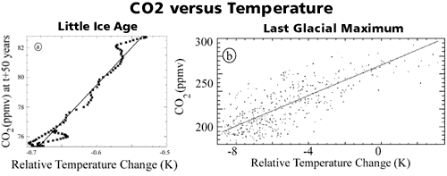
CO2 vs Temperature: Little Ice Age and Last Glacial Maximum
Figure 1. Relationships between past atmospheric CO2 concentrations and reconstructed temperatures. (a) Reconstructed Northern Hemisphere temperatures of the period 1500-1600 plotted against CO2 levels 50 years later from the Law Dome record. (b) CO2 vs temperature for a 400.000 years period of glacial cycles reconstructed from the Vostok ice core.

Over these periods, changes in CO2 are assumed to be primarily driven by temperature. This is because mechanisms other than changing CO2 (such as changes in solar output) drove temperature over these periods. So looking at Figure 1, we can calculate the effect that temperature change has on CO2 levels. However, this is complicated by the fact that different carbon cycle processes operate on different time scales. On a time scale of years, warming has an effect of around 3 ppm of CO2 per degree Celsius. On a scale of centuries, the effect is much larger - around 20 ppm of CO2 per degree Celsius.

What we're interested in is the expected global warming by the end of the 21st century so century time-scales are the focus. The most important period for estimating sensitivity of CO2 to temperature on century time-scales is the Little Ice Age. Figure 1a shows how CO2 levels dropped (with a time lag of 50 years) in response to the drop in temperature in this period. From this is calculated a positive feedback of between 15 to 78% on a century-scale.

The benefit of this study is it provides an independent, empirical method of calculating the positive feedback from the CO2 lag. These results are consistent with what's been found in simulation studies. So when someone mentions to you that CO2 lags temperature, remind them they're actually invoking evidence for a positive feedback that further increases global warming by an extra 15 to 78%.

0 0

Printable Version  |  Link to this page

Comments

Prev  1  2  

Comments 51 to 57 out of 57:

  1. I think there's a misunderstanding between you guys. Someone is talking about "f" and other about "x" like in the series 1+x+x^2+... The two are related by f=1/(1-x), as repeatedly stated by others. Beware that this is valid only for x<1. In this notation you have positive feedbacks when f>1 or x>0, negative feedbacks when f<1 or x<0. For x>1 f diverges and you have runaway warming. But being these definitions based on the linearization of the response ΔT to forcing F I think their validity breaks down well before x=1.
    0 0
  2. Riccardo at 19:56 PM on 28 May, 2010, we are both talking about "feedback factor", I think. "f" is feedback factor, but "x" refers to what? The equation you quoted above, "f=1/(1-x)" is different, I think, to the one quoted by e at 09:57 AM i.e "In your example, the feedback factor is: 1-(1/1.23)= 0.187" What is the basis for the equation you quoted, do you have a link to where it is explained?
    0 0
  3. johnd, 1/(1-x) is the infinite sum of 1+x+x^2+... for x<1 which gives the feedback factor f. Look at chris comments.
    0 0
  4. johnd - A feedback gain of 'x', for example 0.5, means that a change in temperature of 1 degree C will through some mechanism (such as, say, increased H2O) cause an additional rise of 0.5 degree C. However, now there's an additional temperature change of 0.5, and the feedback on that is * 0.5 = 0.25 additional change, so you have an x^2 term, and so on and so on. Feedback operates on the temp. change, regardless of why it occurs; an initial forcing causes a shift, which causes a feedback, which causes a shift, which causes additional feedback, etc., resulting in the geometric series of 1+x+x^2+x^3+..., which sums to 1/(1-x) as long as -1 < x < 1. That's the stability criteria - each successive feedback is smaller, and there's a finite sum. So the total change from 1.0 degree C forcing, for a feedback of x=0.5, is 1 + 0.5 + 0.25 + 0.125 + 0.0625 + ... = 1/(1-0.5) = 2 degrees C. That's 1.0 in forcing and 1.0 in feedback. For a feedback of 0.25, the total is 1.333..., for a feedback of 0.75, a total of 4.0, and so on. You can Google positive and negative feedback for more details - there's quite a lot of well written stuff out there.
    0 0
  5. Aaannnd - I write too quickly again. The formula should be Forcing/(1-Feedback). Note that negative feedback also goes into this formula: a negative feedback of 0.5 on a forcing of 1.0 results in a 0.6667 total rise; damping the effect. This is actually a fun exercise in Excel - build a column starting with the forcing and with each following (cell = previous cell * feedback). The sum of the forcing and feedback column gives the total feedback out to whatever number of rows you put in - I would suggest 30-40 or so. You can then compare that to "Forcing/(1-Feedback)".
    0 0
  6. johnd, Yeah I think I was using the terms a little differently. In my usage and the equation quoted by others x was the feedback factor and f is the sum of all temperature changes and feedbacks. I'll try it with completely different terminology so it doesn't get confused with the others: In a geometric series, the sum (s) of infinite terms with a ratio (r) between successive terms and r < 1 can be calculated as follows: s = a / (1-r) Where a is the value of the first term (the initial forcing in our examples). This is where the 1/(1-x) equation comes from when we have an initial forcing of 1 degree. It calculates the net temperature change in the system after an initial forcing. In your example the final temperature was 1.23, so s=1.23. From the above equation, we can solve for r with: r = 1 - a/s, which is where I got 1-(1/1.23)=.187, which in your example is the ratio (r) between successive feedbacks in the system. This is the number that needs to be < 1 in order to have a finite net feedback. The point is to show that even if you have an infinite series of feedbacks on feedbacks, as long as the ratio of one feedback to the next is < 1, the net temperature change will not be infinite or "runaway".
    0 0
  7. The discussions of positive and negative feedback only discuss special cases of the process. Much has been written about non-linear feedback systems (undescriptively referred to as chaos theory) and, to my knowledge, no one has mentioned it yet on this topic. If the x-x^2 equation is used, the constant in front has an enormous impact on the behavior of the feedback. One can use the relationship x2 = A * (x1-x1^2) to see this point. If x1 is .5 and A is less than 2, a negative feedback is established, greater than 2 a positive feedback is established and both approach equilibrium. However, if A is set to 3.5 a stable, predictable oscillation will result. Things get interesting, and more real world, if A is set to 3.916. In this case, the time series oscillates totally unpredictably in a chaotic fashion, hence the name. Interestingly this particular pair of initial conditions and constant produces a “stable” zone lasting about nine periods. Other initial conditions than x1 =.5 produce different, but similar results. The point of all this is that it is impossible to model non-linear feedback systems in the chaotic region. Therefore it is very difficult to take any comfort in the validity of any of the climate models since both CO2 and temperature have fluctuated significantly in the past. I could be wrong, but I bet they are, or have been in chaotic regions of oscillations. Weather, climates, and financial markets are all examples of non-linear feedback systems. I once produced a model that predicted the mean and standard deviations of the S&P index for a 50 year period using only two overlapping chaotic attractors (forcing functions). The resulting time series was different, but visually, undistinguishable from the actual results. Most importantly it had NO predictive power!
    0 0
    Moderator Response: Chaos is addressed by the post Climate is chaotic and cannot be predicted.

Prev  1  2  

You need to be logged in to post a comment. Login via the left margin or if you're new, register here.


The Consensus Project Website

THE ESCALATOR

(free to republish)


© Copyright 2024 John Cook
Home | Translations | About Us | Privacy | Contact Us