A detailed look at Hansen's 1988 projections
Posted on 20 September 2010 by dana1981
Hansen et al. (1988) used a global climate model to simulate the impact of variations in atmospheric greenhouse gases and aerosols on the global climate. Unable to predict future human greenhouse gas emissions or model every single possibility, Hansen chose 3 scenarios to model. Scenario A assumed continued exponential greenhouse gas growth. Scenario B assumed a reduced linear rate of growth, and Scenario C assumed a rapid decline in greenhouse gas emissions around the year 2000.
Misrepresentations of Hansen's Projections
The 'Hansen was wrong' myth originated from testimony by scientist Pat Michaels before US House of Representatives in which he claimed "Ground-based temperatures from the IPCC show a rise of 0.11°C, or more than four times less than Hansen predicted....The forecast made in 1988 was an astounding failure."
This is an astonishingly false statement to make, particularly before the US Congress. It was also reproduced in Michael Crichton's science fiction novel State of Fear, which featured a scientist claiming that Hansen's 1988 projections were "overestimated by 300 percent."
Compare the figure Michaels produced to make this claim (Figure 1) to the corresponding figure taken directly out of Hansen's 1988 study (Figure 2).
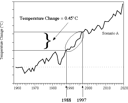
Figure 1: Pat Michaels' presentation of Hansen's projections before US Congress
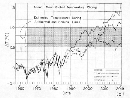
Figure 2: Projected global surface air temperature changes in Scenarios A, B, and C (Hansen 1988)
Notice that Michaels erased Hansen's Scenarios B and C despite the fact that as discussed above, Scenario A assumed continued exponential greenhouse gas growth, which did not occur. In other words, to support the claim that Hansen's projections were "an astounding failure," Michaels only showed the projection which was based on the emissions scenario which was furthest from reality.
Gavin Schmidt provides a comparison between all three scenarios and actual global surface temperature changes in Figure 3.
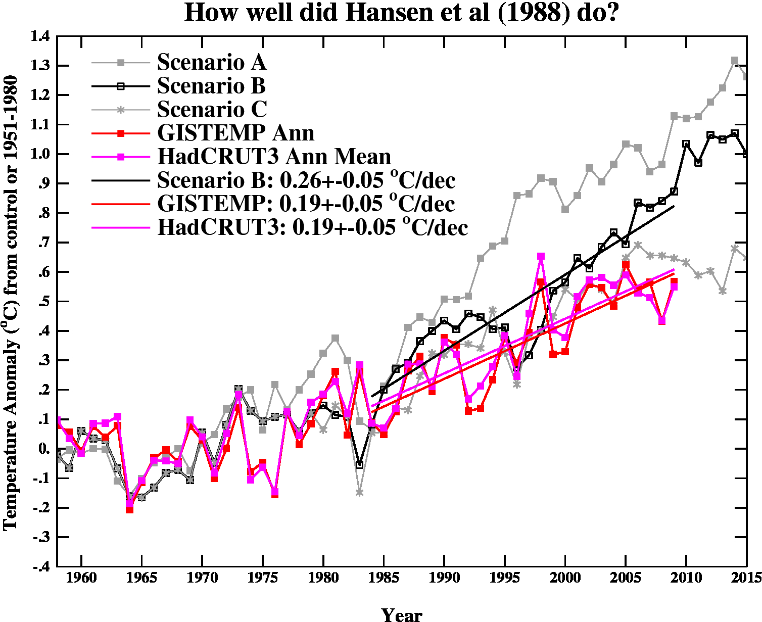
Figure 3: Hansen's projected vs. observed global temperature changes (Schmidt 2009)
As you can see, Hansen's projections showed slightly more warming than reality, but clearly they were neither off by a factor of 4, nor were they "an astounding failure" by any reasonably honest assessment. Yet a common reaction to Hansen's 1988 projections is "he overestimated the rate of warming, therefore Hansen was wrong." In fact, when skeptical climate scientist John Christy blogged about Hansen's 1988 study, his entire conclusion was "The result suggests the old NASA GCM was considerably more sensitive to GHGs than is the real atmosphere." Christy didn't even bother to examine why the global climate model was too sensitive or what that tells us. If the model was too sensitive, then what was its climate sensitivity?
This is obviously an oversimplified conclusion, and it's important to examine why Hansen's projections didn't match up with the actual surface temperature change. That's what we'll do here.
Hansen's Assumptions
Greenhouse Gas Changes and Radiative Forcing
Hansen's Scenario B has been the closest to the actual greenhouse gas emissions changes. Scenario B assumes that the rate of increasing atmospheric CO2 and methane increase by 1.5% per year in the 1980s, 1% per year in the 1990s, 0.5% per year in the 2000s, and flattens out (at a 1.9 ppmv per year increase for CO2) in the 2010s. The rate of increase of CCl3F and CCl2F2 increase by 3% in the '80s, 2% in the '90s, 1% in the '00s, and flatten out in the 2010s.
Gavin Schmidt helpfully provides the annual atmospheric concentration of these and other compounds in Hansen's Scenarios. The projected concentrations in 1984 and 2010 in Scenario B (in parts per million or billion by volume [ppmv and ppbv]) are shown in Table 1.
Table 1: Scenario B greenhouse gas (GHG) concentration in 1984, as projected by Hansen's Scenario B in 2010, and actual concentration in 2010
| GHG |
1984 |
Scen. B 2010 |
Actual 2010 |
| CO2 | 344 ppmv | 389 ppmv | 392 ppmv |
| N2O | 304 ppbv | 329 ppbv | 323 ppbv |
| CH4 | 1750 ppbv | 2220 ppbv | 1788 ppbv |
| CCl3F | 0.22 ppbv | 0.54 ppbv | 0.24 ppbv |
| CCl2F2 | .038 ppbv | 0.94 ppbv | 0.54 ppbv |
We can then calculate the radiative forcings for these greenhouse gas concentration changes, based on the formulas from Myhre et al. (1998).
dF(CO2) = 5.35*ln(389.1/343.8) = 0.662 W/m2
dF(N2O) = 0.12*(![]() N -
N - ![]() N0) - (f(M0,N) - f(M0,N0))
N0) - (f(M0,N) - f(M0,N0))
= 0.12*(![]() 329 -
329 - ![]() 304) - 0.47*(ln[1+2.01x10⁻⁵ (1750*329)0.75+5.31x10⁻¹⁵ 1750(1750*329)1.52]-ln[1+2.01x10⁻⁵ (1750*304)0.75+5.31x10⁻¹⁵ 1750(1750*304)1.52]) = 0.022 W/m2
304) - 0.47*(ln[1+2.01x10⁻⁵ (1750*329)0.75+5.31x10⁻¹⁵ 1750(1750*329)1.52]-ln[1+2.01x10⁻⁵ (1750*304)0.75+5.31x10⁻¹⁵ 1750(1750*304)1.52]) = 0.022 W/m2
dF(CH4) =0.036*(![]() M -
M - ![]() M0) - (f(M,N0) - f(M0,N0))
M0) - (f(M,N0) - f(M0,N0))
= 0.036*(![]() 2220 -
2220 - ![]() 1750) - 0.47*(ln[1+2.01x10⁻⁵ (2220*304)0.75+5.31x10⁻¹⁵ 2220(2220*304)1.52]-ln[1+2.01x10⁻⁵ (1750*304)0.75+5.31x10⁻¹⁵ 1750(1750*304)1.52]) = 0.16 W/m2
1750) - 0.47*(ln[1+2.01x10⁻⁵ (2220*304)0.75+5.31x10⁻¹⁵ 2220(2220*304)1.52]-ln[1+2.01x10⁻⁵ (1750*304)0.75+5.31x10⁻¹⁵ 1750(1750*304)1.52]) = 0.16 W/m2
dF(CCl3F) = 0.25*(0.541-0.221) = 0.080 W/m2
dF(CCl2F2) = 0.32*(0.937-0.378) = 0.18 W/m2
Total Scenario B greenhouse gas radiative forcing from 1984 to 2010 = 1.1 W/m2
The actual greenhouse gas forcing from 1984 to 2010 was approximately 1.06 W/m2 (NASA GISS). Thus the greenhouse gas radiative forcing in Scenario B was too high by about 5%.
Climate Sensitivity
Climate sensitivity describes how sensitive the global climate is to a change in the amount of energy reaching the Earth's surface and lower atmosphere (a.k.a. a radiative forcing). Hansen's climate model had a global mean surface air equilibrium sensitivity of 4.2°C warming for a doubling of atmospheric CO2 [2xCO2]. The relationship between a change in global surface temperature (dT), climate sensitivity (λ), and radiative forcing (dF), is
dT = λ*dF
Knowing that the actual radiative forcing was slightly lower than Hansen's Scenario B, and knowing the subsequent global surface temperature change, we can estimate what the actual climate sensitivity value would have to be for Hansen's climate model to accurately project the average temperature change.
Actual Climate Sensitivity
One tricky aspect of Hansen's study is that he references "global surface air temperature." The question is, which is a better estimate for this; the met station index (which does not cover a lot of the oceans), or the land-ocean index (which uses satellite ocean temperature changes in addition to the met stations)? According to NASA GISS, the former shows a 0.19°C per decade global warming trend, while the latter shows a 0.21°C per decade warming trend. Hansen et al. (2006) – which evaluates Hansen 1988 – uses both and suggests the true answer lies in between. So we'll assume that the global surface air temperature trend since 1984 has been one of 0.20°C per decade warming.
Given that the Scenario B radiative forcing was too high by about 5% and its projected surface air warming rate was 0.26°C per decade, we can then make a rough estimate regarding what its climate sensitivity for 2xCO2 should have been:
λ = dT/dF = (4.2°C * [0.20/0.26])/0.95 = 3.4°C warming for 2xCO2
In other words, the reason Hansen's global temperature projections were too high was primarily because his climate model had a climate sensitivity that was too high. Had the sensitivity been 3.4°C for a 2xCO2, and had Hansen decreased the radiative forcing in Scenario B slightly, he would have correctly projected the ensuing global surface air temperature increase.
The argument "Hansen's projections were too high" is thus not an argument against anthropogenic global warming or the accuracy of climate models, but rather an argument against climate sensitivity being as high as 4.2°C for 2xCO2, but it's also an argument for climate sensitivity being around 3.4°C for 2xCO2. This is within the range of climate sensitivity values in the IPCC report, and is even a bit above the widely accepted value of 3°C for 2xCO2.
Spatial Distribution of Warming
Hansen's study also produced a map of the projected spatial distribution of the surface air temperature change in Scenario B for the 1980s, 1990s, and 2010s. Although the decade of the 2010s has just begun, we can compare recent global temperature maps to Hansen's maps to evaluate their accuracy.
Although the actual amount of warming (Figure 5) has been less than projected in Scenario B (Figure 4), this is due to the fact that as discussed above, we're not yet in the decade of the 2010s (which will almost certainly be warmer than the 2000s), and Hansen's climate model projected a higher rate of warming due to a high climate sensitivity. However, as you can see, Hansen's model correctly projected amplified warming in the Arctic, as well as hot spots in northern and southern Africa, west Antarctica, more pronounced warming over the land masses of the northern hemisphere, etc. The spatial distribution of the warming is very close to his projections.
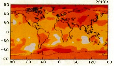

Figure 4: Scenario B decadal mean surface air temperature change map (Hansen 1988)
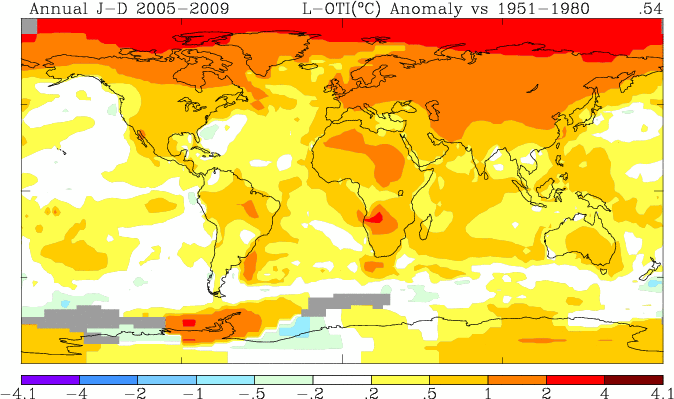
Figure 5: Global surface temperature anomaly in 2005-2009 as compared to 1951-1980 (NASA GISS)
Hansen's Accuracy
Had Hansen used a climate model with a climate sensitivity of approximately 3.4°C for 2xCO2 (at least in the short-term, it's likely larger in the long-term due to slow-acting feedbacks), he would have projected the ensuing rate of global surface temperature change accurately. Not only that, but he projected the spatial distribution of the warming with a high level of accuracy. The take-home message should not be "Hansen was wrong therefore climate models and the anthropogenic global warming theory are wrong;" the correct conclusion is that Hansen's study is another piece of evidence that climate sensitivity is in the IPCC stated range of 2-4.5°C for 2xCO2.
This post is the Advanced version (written by dana1981) of the skeptic argument "Hansen's 1988 prediction was wrong". After reading this, I realised Dana's rebuttal was a lot better than my original rebuttal so I asked him to rewrite the Intermediate Version. And just for the sake of thoroughness, Dana went ahead and wrote a Basic Version also. Enjoy!


 Arguments


- Scenario C provides a better prediction of real temperatures than Scenario B.
- The Scenario C warming trend for 1984-2009 is 0.24 °C/dec. This is near to the measured rate of 0.19 °C/dec and is significantly closer to reality than the Scenario B rate of 0.26 °C/dec.
- The Scenario C prediction for 2000-2019 is nearly zero at 0.01 °C/dec. Furthermore, for the ten years that have elapsed since 2000, it appears to be “on the money.”
CONCLUSIONS Hansen and his 1988 team are to be commended for producing models that are close to reality. Scenario C in particular has shown significant skill in predicting actual temperatures. Additionally, Hansen’s (2006) comments on the 1988 models that,“… a 17-year period is too brief for precise assessment of model predictions, but distinction among scenarios [B & C] and comparison with the real world will become clearer within a decade [2015].” I concur, let us wait until 2015 to see which scenario is correct. Will the “black box" that is Scenario C be right or will the real world move closer to Scenario B?Some of your graphics are innacurate. Here is Hansen's model compared to actual temperatures:
IPCC prediction and reality:
Taken from here: https://mises.org/daily/5892/The-Skeptics-Case
Wow, that's quite an iulluminating comment, applebloom.
First, you graph a prediction of surface temperature agains satellite data, which is not a surface temperature. Strike 1.
Then you use a graph that shifts the prediction up to match a high spike from 1988 in noisy data, to maximize the chance that later data will fall below the prediction. Strike 2.
Then you provide a graph that looks like it has taken a 100-year IPCC scenario result and treated the value is if it is linear over the period, and claim it's too high. Strike 3.
Did you apply any skepticism to that source at all? Or did you just accept it hook, line, and sinker?
Bob Loblaw @130, you missed the outragious claim that Scenario A was what "actually occurred". Given that CO2 concentrations, as indeed all other GHG concentrations were still below the Scenario B values in 2010, and the total GHG forcing was less than that in scenario B, such a claim cannot have been honestly made. It was either made in ignorance of the data, and hence what actually happened, and is dishonest in implicitly claiming that knowledge, or it is more directly dishonest in that the person making the claim knew it to be false when they made it. As you say, very illuminating.
"Some of your graphics are innacurate". That would be one of the funnier comments we have seen.
And add that he used UAH satellite data rather than the results from RSS that show nerly twice as much warming.
Sometimes ya just gotta luv how creative some skeptics can be with data. Cherry farmers every single one of them.
I would like to see these graphs updated to 2015 and have the discussion again.
I too would like to see an update of this topic, afterall comparing the 'guess' with observation is the foundation of the scientific method.